
Topic 6: Heat Engines#
Introduction#
As we saw in example 5.1, tracing out a closed cycle on a \(PV\) plot can result in a partial conversion of heat into work (only partial, because not all the heat supplied is converted: some is output as waste heat). Macroscopic kinetic energy is energy associated with organized, coordinated motions of many molecules, whereas heat transfer involves changes in energy of disordered molecular motion. Conversion of mechanical energy into heat involves an increase of disorder. As a prelude to the second law of thermodynamics we will consider two classes of device: heat engines are partly successful in converting heat into work. Refrigerators are partly successful in transporting heat from cooler to hotter bodies.
A heat engine is any device that takes in heat \(Q_H\), converts some of it into work \(W\), and outputs the rest as waste heat \(Q_C\) . The engine contains a working fluid that undergoes various processes (heating, cooling, compression, expansion) in the course of the cycle. In the heat engines we shall consider in this course, we will assume that the working fluid is an ideal gas and that all the processes involved are quasistatic and reversible. In real engines, this is not true: many real engine cycles, such as the steam engine, rely in part on a phase change (the working fluid of a steam engine is water, which spends part of the cycle as liquid water, part as water vapour, and part as liquid and vapour in equilibrium), which means that the working fluid cannot be modelled as an ideal gas, and of course all real engines lose some energy to irreversible processes such as friction. However, a number of common engines can be reasonably well modelled as a cycle of reversible processes applied to an ideal gas as working fluid, and we shall look at some of these in this section.
Thermal efficiency of a heat engine#
The thermal efficiency of a heat engine, usually denoted \(\eta\), is the fraction of the input heat that is converted into work in one complete cycle
Here I have written \(|W|\), because our First Law definition of \(W\) is the work done on the system, and the purpose of a heat engine is to do work, so we expect \(W < 0\). Since the engine returns to its initial state at the end of each cycle, and we know that \(U\) is a function of state, we must have \(\Delta U = 0\) at the end of a cycle, and therefore \(\Delta Q = Q_{H} - |Q_{C}| = |W|\). Again we write \(|Q_{C}|\) because we defined \(Q_{C}\) above as the heat given out by the system, whereas in our definition of the First Law \(Q\) us always heat supplied to the system. Substituting this into Equation (30) gives
Obviously the aim of engine designers is to maximise \(\eta\).
Fig. 11 shows the operation of a petrol engine. First a mixture of air and petrol vapour flows into a cylinder through an open intake value while the piston descends, increasing the volume of the cylinder from a minimum of \(V\) (when the piston is all the way up) to a maximum of \(rV\) (when it is all the way down). The quantity \(r\) is called the compression ratio. At the end of this intake stroke, the intake value closes and the mixture is compressed to volume \(V\) during the compression stroke. The mixture is then ignited by the spark plug, and the heated gas expands back to volume \(rV\), pushing on the piston and doing work; this is the power stroke. Finally the exhaust valve opens, and the combustion products are pushed out (during the exhaust stroke), leaving the cylinder ready for the next intake stroke.
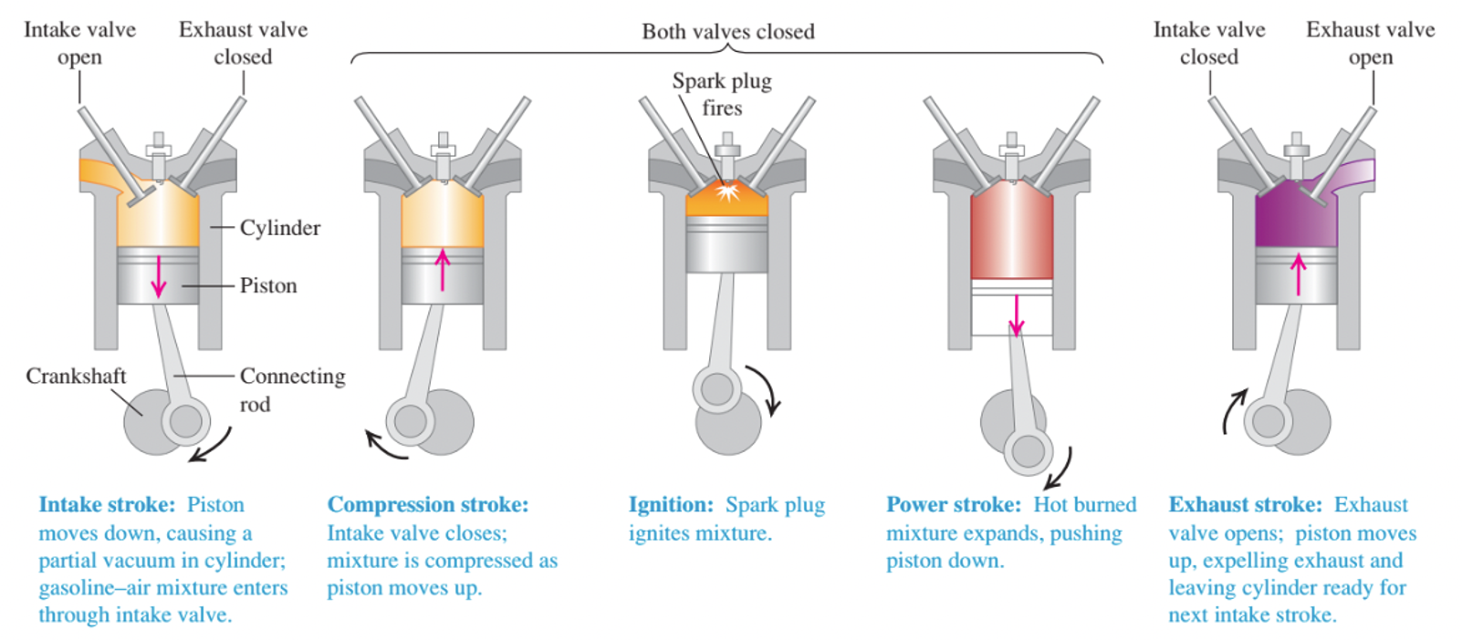
Fig. 11 Cycle of an internal-combustion engine. Source: Fig 20.5 from University Physics with Modern Physics (Pearson)#
Some idealised heat engines#
The Otto cycle#
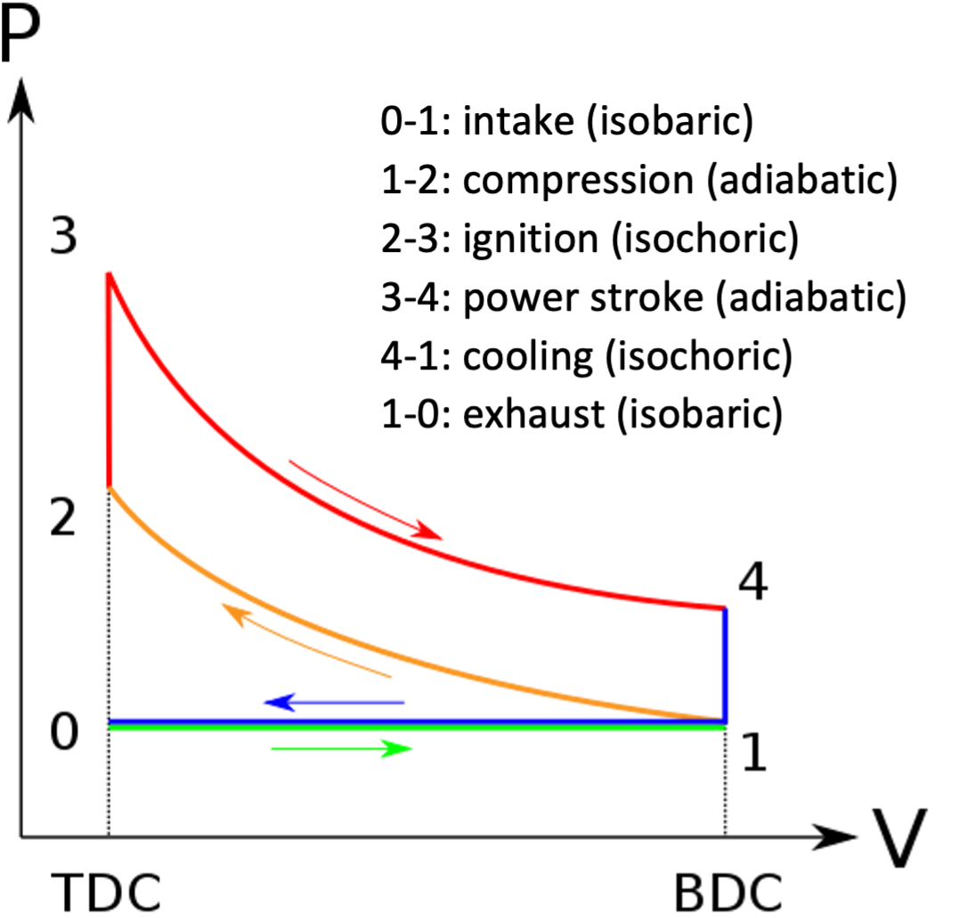
The Otto cycle is an idealised version of the petrol engine. As shown in Fig. 12, the Otto cycle consists of six processes, but the first and last do not affect the work done or the efficiency, and can be neglected.
In the Otto cycle, heat is added at constant volume in step 2-3 (this represents the injection and ignition of the fuel) and rejected at constant volume in step 4-1 (when the exhaust valve is opened). Work is done adiabatically on the gas in step 1-2 as the piston moves up from BDC (bottom dead centre) to TDC (top dead centre), and by the gas as it forces the piston back out in step 3-4. Although we think of a petrol engine as being driven by petrol, the working fluid is actually air, or more precisely a mixture of air and combustion products: the petrol powers the engine by supplying the input heat in step 2-3.
From Equation (31), the efficiency of the Otto engine is \(\eta = 1 - \frac{T_4 - T_1}{T_3 - T_2}\), since the heat supplied at constant volume is \(Q = C_{V} \Delta T\) and we assume that \(C_{V}\) is the same in both steps (note that in a real engine it won’t be, since the working gas has a different chemical composition after ignition).
Since steps 1-2 and 3-4 are both adiabatic, we know from Equation (27) that \(T_{4} V_{1}^{\gamma -1} = T_{3} V_{2}^{\gamma - 1}\) and \(T_{1} V_{1}^{\gamma -1} = T_{2} V_{2}^{\gamma - 1}\). Therefore we can write \(T_{4} - T_{1} = T_{3} \left( \frac{V_{2}}{V_{1}}\right)^{\gamma-1} - T_{2} \left (\frac{V_{2}}{V_{1}}\right)^{\gamma-1} = (T_{3} - T_{2}) \left( \frac{V_{2}}{V_{1}} \right)^{\gamma-1}\), and hence we can simplify the efficiency to
where \(r = V_{1} / V_{2}\) is the compression ratio. Therefore, to maximise the efficiency of a petrol engine, we should aim to maximise the compression ratio. This is limited by the fact that \(T_{2} = T_{1} r^{\gamma-1}\): if we increase the compression ratio too much, the temperature inside the cylinder will increase to the point where the fuel ignites prematurely, before the spark. Typical compression ratios for petrol engines are around 10:1 (between 8:2 and 12:1).
Example 6.1
Calculate the theoretical efficiency of an Otto-cycle engine with \(r\)=9.5 and \(\gamma\)=7/5. If the engine takes in 10 kJ of heat from burning its fuel, how much heat does it discard to the outside air?
\(\eta = 1 - \frac{1}{r^{\gamma-1}}\) = 0.59 or 59%. \(Q_{C} = (1 - \eta) Q_{H}\) = 4.1 kJ.
Diesel cycle#
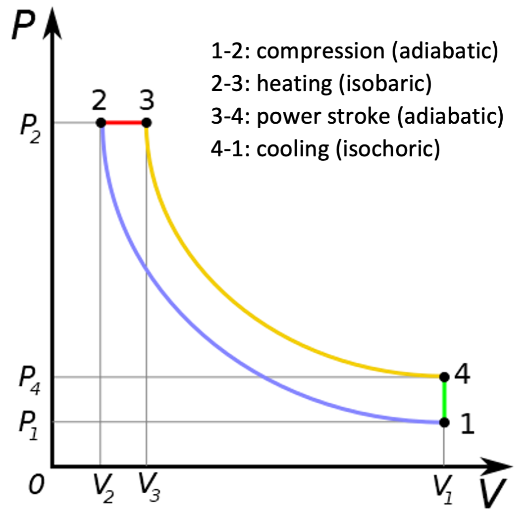
The Diesel cycle, as its name suggests, is an idealised version of the diesel engine. The difference between the Diesel cycle and the Otto cycle is that the heating stage 2-3 takes place at constant pressure, rather than at constant volume as in the Otto cycle. The intake stroke (step 0-1) and exhaust stroke (step 4-0) shown in Fig. 12 do exist in the Diesel cycle, but have been omitted from Fig. 13.
The thermal efficiency of a diesel engine is given by \(\eta = 1 - \frac{C_{V} (T_{4} - T_{1})}{C_{P} (T_{3} - T_{2})}\). This is more complicated to work out than the petrol engine, because there are three volumes involved instead of two. We define the compression ratio \(r = V_{1} / V_{2}\) as before, and also the cut-off ratio, \(\alpha = V_{3} / V_{2}\). From the ideal gas law we deduce that it is also true that \(\alpha = T_{3} / T_{2}\).
From step 3-4 we deduce that \(T_{4} V_{1}^{\gamma-1} = T_{3} V_{3}^{\gamma-1} = (\alpha T_{2}) (\alpha V_{2})^{\gamma-1} = \alpha^{\gamma} T_{2} V_{2}^{\gamma-1}.\) From step 1-2 we have \(T_{1} V_{1}^{\gamma-1} = T_{2} V_{2}^{\gamma-1}\), so \(T_{4} - T_{1} = \left( \frac{V_{2}}{V_{1}}\right)^{\gamma-1} (\alpha^{\gamma} - 1) T_{2} = \frac{\alpha^{\gamma} - 1}{r^{\gamma-1}} T_{2}\) and \(T_{3} - T_{2} = (\alpha -1) T_{2}\); Hence
How does this compare with the efficiency of the Otto cycle?
If we write \(\beta = \alpha -1\) then \(\alpha^{\gamma} = (1+\beta)^{\gamma} = 1 + \gamma \beta + \frac{1}{2} \gamma (\gamma - 1) \beta^{2} + \cdots > 1 + \gamma \beta,\) since both \(\alpha\) and \(\gamma\) are greater than 1. Therefore
so for the same compression ratio, \(r\), the Otto cycle has a higher efficiency than the Diesel cycle. However, in practice diesel engines can run at higher compression ratios than petrol engines (between 14:1 and 23:1, so roughly double a typical petrol engine compression ratio), and the factor \(\frac{\alpha^{\gamma} - 1}{\gamma(\alpha-1)}\) is not very much greater than 1 (typical values of \(\alpha\) seem to be around 2, which for a diatomic working gas with \(\gamma\) = 7/5 gives 1.17), so a typical diesel engine is likely to be more efficient than a typical petrol engine.
The value of \(\alpha\) is constrained by \(T_{3}\), which is set by the temperature at which the fuel will ignite: unlike a petrol engine, diesel engines have no need for spark plugs since the full ignites spontaneously when it reaches the appropriate temperature. Since \(T_{2}/T_{1} = r^{\gamma -1}\), we can express \(\alpha\) in terms of the compression ratio, \(T_{1}\) and \(T_{3}\) by
As \(T_{1}\) and \(T_{3}\) are reasonably well defined, this means that the cut-off ratio is not really an independent parameter; if we know the flame temperature \(T_{3}\) and the inlet temperature \(T_{1}\), it is set by the compression ratio.
Example 6.2
A Diesel engine performs 2.2 kJ of mechanical work and discards 4.3 kJ of heat each cycle. (i) How much heat is supplied to the engine each cycle? (ii) What is the thermal efficiency of the engine?
(i) Work done by the engine is 2200 J so work done on engine is \(W\) = -2200 J. Heat given out by engine is 4300 J so \(Q_{C}\) = -4300 J therefore \(Q_{H} = |W| + |Q_{C}|\) = 6500 J.
(ii) \(\eta = \frac{|W|}{Q_{H}} = \frac{2200}{6500} = 0.34\) or 34%.
Stirling cycle#
Unlike the Otto and Diesel cycles, the Stirling cycle relates to an external combustion engine, where the heat is supplied from an external heat reservoir. This has the advantage that the engine can use a very wide range of heat sources, since the fuel never comes into contact with the working gas. The disadvantage is that the heat needs to be transported from the external reservoir to the working fluid via some sort of heat exchanger, which is likely to reduce the efficiency of real Stirling engines compared to the idealised model described here.
The Stirling cycle is more complicated to analyse than the Otto or Diesel cycles, because the compression and power strokes are isothermal rather than adiabatic, so heat is supplied or rejected in all four steps.
Step 1-2: work done on system \(W_{12} = n R T_{C} \ln (V_{1}/V_{2})\). As this step is isothermal, \(\Delta U = 0\) and so the system must output heat \(|Q_{12}| = n R T_{C} \ln (V_{1}/V_{2})\).
Step 2-3: isochoric heating, so no work done and the system takes in heat \(Q_{23} = n c_{V} (T_{H} - T_{C})\).
Step 3-4: work done by system \(|W_{34}| = n R T_{H} \ln (V_{1}/V_{2})\). Since \(\Delta U = 0\), the system must take in heat \(Q_{34} = n R T_{H} \ln (V_{1}/V_{2})\).
Step 4-1: isochoric cooling: no work, and the system outputs heat \(|Q_{41}| = n c_{V} (T_{H} - T_{C}).\)
The net work done by the system is therefore \(|W| = |W_{34}| - W_{12} = n R (T_{H} - T_{C}) \ln (V_{1}/V_{2})\), and the heat supplied is \(Q_{H} = Q_{23} + Q_{34} = n(c_{v} (T_{H} - T_{C}) + R T_{H} \ln (V_{1}/V_{2}))\). Therefore the efficiency of the cycle is, from Equation (30).
However, this is not the whole story. The Stirling engine is a regenerative engine: the heat released in step 4-1 is stored in a heat exchanger and used to reheat the working gas in step 2-3. If this is perfectly efficient (which, of course, it won’t be in the real world), steps 2-3 and 4-1 cancel each other out, and we have
We shall see later that this is in fact the theoretical maximum for the efficiency of a heat engine. As one would expect, this is not achieved in real-world Stirling engines (no real engine is as efficient as the idealised cycles we have been considering here, but the difference between real and idealised Stirling engines is greater than most). However, real Stirling engines do have good efficiency, comparable with diesel engines.
Unlike internal-combustion engines, Stirling engines are genuinely reversible: instead of using the heat difference between the two reservoirs to generate mechanical work, mechanical work can be supplied to transfer heat from the cold reservoir to the hot reservoir. This is not used in domestic refrigerators, because cycles involving phase changes are more cost-effective, but is widely used in cryocoolers (i.e. refrigerators working at temperatures below about -40\(^{\circ}\) C).
Stirling engines are also very quiet, and have been used in submarines for this reason.
Brayton cycle#
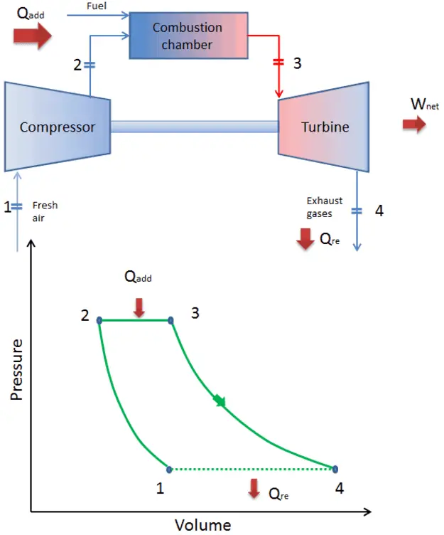
Fig. 15 The (open) Brayton cycle. Source: www.nuclear-power.com#
The Brayton cycle describes the workings of a constant-pressure heat engine. Examples include jet engines (open cycle) and gas turbines in power stations (closed cycle). A schematic of the open Brayton cycle is shown in Fig. 15. The four steps of the Brayton cycle are
1-2: Adiabatic compression (air compressed to high pressure and temperature within inlet and compressor)
2-3: Isobaric heat addition (via burining fuel-air mix in combustion chamber)
3-4: Adiabatic expansion (combustion products expand in the turbine and exhaust nozzle)
4-1: Isobatic heat rejection (gas discharged into atmosphere, cooled back to initial condition)
The thermal efficiency of the Brayton cycle can be expressed in terms of the compressor temperature ratio
and subsequently in terms of the compressor pressure ratio using the relationship between temperature and pressure for adiabatic processes
so higher efficiency is achieved at high pressure ratios (30-40 for modern engines), subject to limits set by the maximum temperature that the turbine blades can withstand (approx 1700 K).
The Carnot cycle: the ‘perfect’ heat engine#
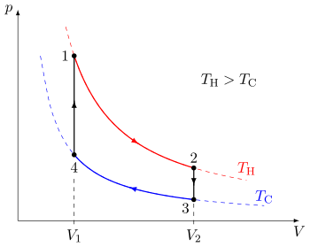
The best possible cycle for a heat engine was proposed in 1824 by the French physicist Sadi Carnot (1796-1832). The Carnot cycle is shown in Fig. 16: it consists of two adiabatic steps and two isothermal steps. Heat is supplied in step 3-4 and rejected in step 1-2: work is done in all four steps. Only two temperatures are involved: \(T_{3} = T_{4} = T_{H}\) and \(T_{1} = T_{2} = T_{C}\).
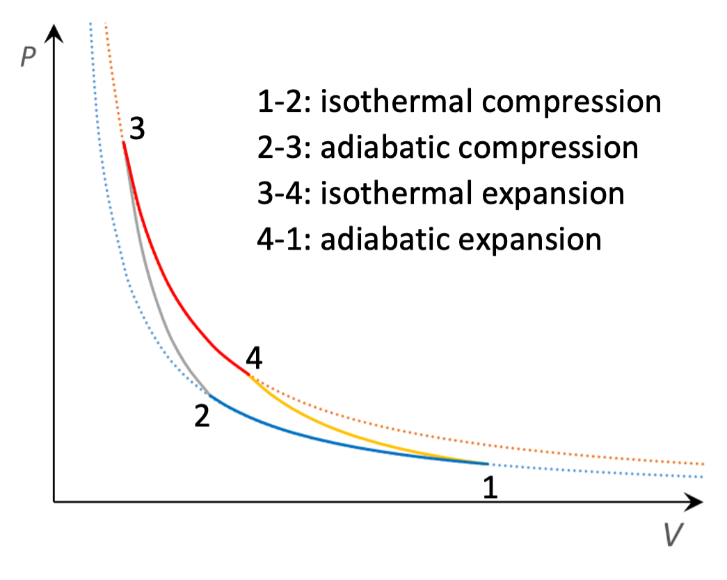
Fig. 16 The Carnot cycle.#
Taking each step in turn:
Step 1-2, work done on system \(W_{12} = n R T_{C} \ln (V_{1} / V_{2})\). As this step is isothermal \(\Delta U = 0\) and so the system must output heat \(|Q_{12}| = n R T_{C} \ln (V_{1} / V_{2})\).
Step 2-3: as this step is adiabatic, the heat supplied is zero, and from Equation (29), the work done is \(W_{23} = \frac{1}{\gamma-1} (P_{3} V_{3} - P_{2} V_{2}) = n c_{V} (T_{H} - T_{C})\).
Step 3-4: work done by system \(|W_{34}| = n R T_{H} \ln (V_{4} / V_{3})\). Since \(\Delta U = 0\), the system must take in heat \(Q_{34} = n R T_{H} \ln (V_{4}/ V_{3})\).
Step 4-1: the work done by the system is \(|W_{41}| = n c_{V} (T_{H} - T_{C}).\) As the same temperatures are involved as in step 2-3 these just cancel out so the net work done by the system is \(|W_{34}| - W_{12}\).
To simplify the resulting expression we use Equation (27) to deduce \(V_{2} T_{C}^{\gamma-1} = V_{3} T_{H}^{\gamma-1}\) and \(V_{1} T_{C}^{\gamma-1} = V_{4} T_{H}^{\gamma-1}\). Therefore we conclude that \(V_{1}/V_{2} = V_{4}/V_{3}\). Hence the net work done by the system is \(|W| = n R (T_{H} - T_{C}) \ln (V_{4}/V_{3})\), and the heat supplied is \(Q_{H} = Q_{34} = n R T_{H} \ln (V_{4}/V_{3})\). From Equation (30) the efficiency of the Carnot cycle is
The Carnot cycle is not an idealised version of a real engine - in practical terms it is extremely difficult to supply heat without raising the temperature of your working fluid. It was deliberately designed as a theoretical construct to demonstrate maximum efficiency. We shall see in the next section that the Second Law of Thermodynamics can be used to demonstrate that it is impossible for any engine, real or idealized, to be more efficient than a Carnot engine.
Equation (35) can be used to define the thermodynamic temperature, because although we used the ideal gas law to derive it, it is in fact indepedent of the working substance of the cycle. Therefore, if a Carnot cycle takes in heat \(Q_{H}\) and rejects heat \(|Q_{C}|\), we can define the Kelvin temperature
Since the Carnot cycle is purely theoretical and does not correspond to any real device, this is not a very useful definition in practical terms, but it is closely connected to the definition of temperature in terms of entropy, which is useful.
Example 6.3
A Carnot engine, whose high temperature reservior is at 620 K, takes in 550 J of heat at this temperature in each cycle and gives up 335 J to the low temperature reservoir. (i) How much mechanical work does the engine perform during each cycle? (ii) What is the temperature of the low temperature reservoir? (iii) What is the thermal efficiency of the cycle?
(i) \(|W| = Q_{H} - |Q_{C}|\) = 550 - |-335| = 215 J.
(ii) \(T_{C} = \frac{|Q_{C}|}{Q_{H}} T_{H} = \frac{|-335|}{550} \times 620 = 378\) K
(iii) \(\eta = 1 - \frac{T_{C}}{T_{H}} = 1 - \frac{378}{620} = 0.39\) or 39%.
Example 6.4
You design an engine that takes in \(1.5 \times 10^{4}\) J of heat at 650 K in each cycle and rejects heat at 350 K. The engine completes 240 cycles in 1 minute. What is the theoretical maximum power output of your engine in hp? (1 hp = 746 W)
For an idealised (Carnot) engine, \(\eta = 1 - \frac{T_{C}}{T_{H}} = 1 - \frac{350}{650} = 0.46 \) or 46%.
\(|W| = \eta Q_{H} = 0.46 \times 1.5 \times 10^{4} = 6900\) J. 240 cycles per minute corresponds to 4 cycles per second. Power (P) is work done per cycle (W) times number of cycles (per second), so \(P = 6900 \times 4 = 26.7\) kW or 37 hp.
A two-phase heat engine#
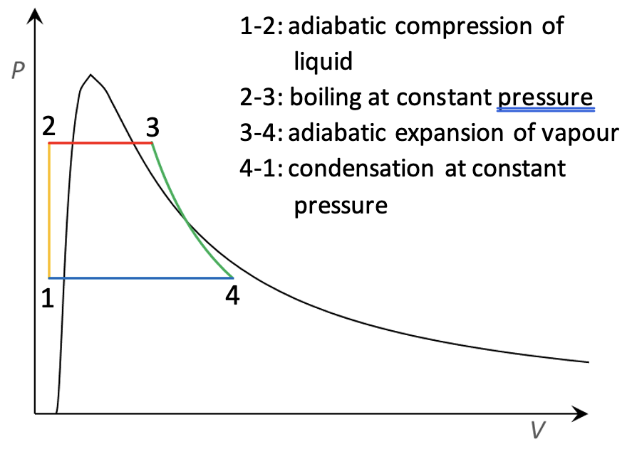
Fig. 17 Rankine cycle#
Thermodynamics was invented in the age of the steam engine, so unsurprisingly there is a thermodynamic cycle representing the idealised steam
engine. This is the Rankine cycle (see Fig. 17), developed in the 1850s by the Scottish physicist William Rankine (1820-1872).
The Rankine cycle differs from those discussed above in that it involves a phase change: the working fluid (water in steam engines) is
liquid for part of the cycle. Obviously this cannot be represented by an ideal gas, because the ideal gas law does not model phase changes.
In Fig. 17, the area to the left of the black curve is the liquid state, to the right is gas, and under the curve is a mixture of gas and liquid in equilibrium. The cycle consists of four processes:
Step 1-2: the working fluid, in the liquid state, is pumped from low to high pressure. This is an adiabatic compression, but because liquids are nearly incompressible there is very little change of volume and therefore very little work done.
Step 2-3: the high-pressure liquid is heated at constant pressure. It boils and becomes a dry vapour (the word dry means that there are no liquid droplets remaining).
Step 3-4: the vapour expands adiabatically. This is the power stroke which does the useful work. As the vapour cools during the expansion, some liquid droplets may form (making it a wet vapour).
Step 4-1: the vapour is cooled at constant pressure, condensing back into a liquid.
The Rankine engine is an external combustion engine, using an external heat source in step 2-3 (in a steam locomotive, it’s the fire under the boiler). Although steam engines are no longer used in transport, the Rankine cycle also describes steam turbines, which are used in power stations to generate electricity from heat. As with the Stirling engine, the Rankine engine is not dependent on any particular fuel.
The advantage of the two-phase operation is that the initial adiabatic heating requires very little work: the power required by the pump is only 1–3% of the turbine output power. If this were done in the gas phase, the power required to drive the pump would be substantially greater.
Refrigerators and heat pumps#
A heat engine takes in heat from a hot reservoir, converts some of it to mechanical work and rejects the rest to a cold reservoir. Our idealised cycles all use reversible processes, so we should be able to run them in reverse. In reverse, the working fluid takes in heat from a cold reservoir, some work is done on it, and the resulting (greater) heat is expelled into a hot reservoir. The net effect of doing work on the system is to move heat from the cold reservoir to the hot reservoir - in other words, it’s a refrigerator. (A heat pump is thermodynamically equivalent to a refrigerator, but it has a different purpose: the aim of a refrigerator is to cool the cool reservoir; i.e. the interior of the fridge, whereas the aim of a heat pump is to heat the hot reservoir, i.e. the interior of the building).
Real internal combustion engines are not reversible, because the heating stage (step 2-3 in the Otto and Diesel cycles) is achieved by igniting the fuel, which is not a reversible procedure. External combustion engines, such as the Stirling and Rankine cycles, are much more promising. Domestic fridges use a reverse Rankine cycle, as shown schematically in Fig. 18.
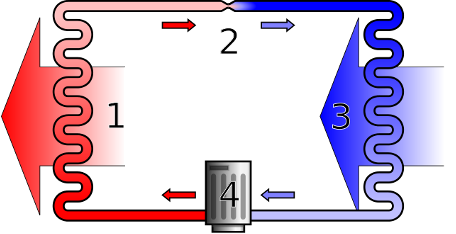
Fig. 18 Schematic diagram of a heat pump or refrigerator. Source: Wikipedia#
In Fig. 18 hot vapour enters the condenser (1), where it is condensed into a liquid, releasing heat (corresponding to steps 3-2 in Fig. 17). The resulting high-pressure liquid flows through an expansion valve (2), which causes a drop in pressure and temperature (steps 2-1 in Fig. 17). The cold, low pressure fluid (a mixture of liquid and vapour) then passes through the evaporator (3) where it is converted to a vapour, taking in heat from its surroundings (steps 1-4 in Fig. 17). It then passes to the compressor (4) where it is pumped up to a high pressure (with a consequent increase in temperature) to return to the initial stage (steps 4-3 in Fig. 17).
The equivalent of efficiency for a refrigerator or heat pump is called the coefficient of performance. This is defined broadly as the ratio of the desired output to the work done, which means that it is different for refrigerators and heat pumps. For a refrigerator the desired output is the removal of heat from the cold reservoir, so the coefficient of performance is
whereas for a heat pump the desired output is the supply of heat to the hot reservoir, so
From the first law, \(W = |Q_{H}| - Q_{C}\), giving
If the refrigerator cycle were an ideal cycle with thermal efficiency \(\eta= 1 - T_{C}/T_{H}\) the coefficients of performance would be
Notice that these are typically greater than one. For example, if your kitchen has a temperature of 25\(^{\circ}\) C and you want your fridge to be at 4\(^{\circ}\) C, the ideal coefficient of performance would be 277/21 = 13.2; conversely if your kitchen is heated to 25\(^{\circ}\) C by a heat pump operating between the house and outside air with a temperature of 4\(^{\circ}\) C the ideal coefficient of performance would be 298/21 = 14.2. These values represent the maximum theoretically achievable, and in the real world coefficients of performance will be substantially less than this, especially for heat pumps since one should take into account the power required to circulate the heat around the house e.g. by pumping hot water through the radiator system, However, even real coefficients of performance are significantly greater than unity.
Example 6.5
A refrigerator has a coefficient of performance of 2.1. In each cycle it absorbs \(3.4 \times 10^{4}\) J of heat from the cold reservoir. (a) How much mechanical energy is required each cycle to operate the refrigerator? (b) During each cycle how much heat is discarded to the high temperature reservoir?
(a) \(COP_{R} = Q_{C}/W\) so \(W = Q_{C}/COP_{R} = 3.4\times 10^{4}/2.1 = 16.2\) kJ.
(b) \(COP_{R} = Q_{C}/(Q_{H} - Q_{C})\) so \(Q_{H} = Q_{C}(1 + 1/COP_{R}) = 3.4\times 10^{4} (1 + 1/2.1) = 50.2\) kJ.