Topic 3: The Ideal Gas

Introduction

Many applications of thermodynamics involve gases. The working fluids of most engines are gases (steam, petrol or diesel vapour, etc.); most astrophysical objects are gaseous; atmospheric physics obviously relates mainly to gases. It is therefore important to have an effective model of a gas. As is often the case in physics, our usual working model is a simplified system known as an ideal gas; fortunately, many real gases are very good approximations to the ideal gas.

Our picture of an ideal gas relies on kinetic theory, which was developed in the 19th century by pioneers of thermal physics such as Rudolf Clausius, James Clerk Maxwell and Ludwig Boltzmann. This was an early application of the atomic theory of matter, since kinetic theory relies on the assumption that a gas consists of very large numbers of small particles in random motion.

The definition of an ideal gas

The description of a gas in kinetic theory relies on the following assumptions:

• the gas particles are small enough that they can be treated as points - i.e., the volume taken up by the particles themselves is negligible compared to the volume occupied by the gas;

• the particles are in constant random motion and obey Newton’s laws;

• all collisions between particles, or between a particle and a wall of the container, are perfectly elastic;

• forces between particles are negligible except during collisions.

In addition, it is assumed that there are so many particles that it is justified to work in terms of statistical averages. Many of the properties of a gas, particularly pressure and temperature, are averages: it would be impossible to define the pressure or temperature of a gas consisting of only one particle.

Example 3.1

Question

The core of the Sun consists mostly of completely ionized hydrogen and helium; the fraction of helium by mass is approximately 2/3. The temperature and density in this region are \(1.56 \times 10^7\) K and \(1.48 \times 10^5\)
kg/m\(^3\). The radius of the proton is about 1 fm, and the radius of a helium nucleus is about 1.7 fm; the classical electron radius is about 2.8 fm. Is it reasonable to treat the core of the Sun as an ideal gas?

Solution

If the helium fraction is 2/3 by mass, then, given that helium has a mass four times that of hydrogen, there must be 2 hydrogen atoms for every helium. If they are all fully ionized, that means that the particles in the Solar core are in the ratio 4 electrons: 2 protons: 1 helium nucleus ( 2 protons, 2 neutrons). The total mass of one set of particles is 6 \(u\) (= proton mass), since the electron mass is negligible, so the average mass per particle is 6/7 \(u = 1.4 \times 10^{-27}\) kg. This means that there are \(1.48 \times 10^{5} / 1.4 \times 10^{-27} = 1.0 \times 10^{32}\) particles per cubic metre, so each particle occupies a volume of \( 1.0 \times 10^{-32}\) m\(^3\). But the volume actually occupied by each particle, even taking them all to have the volume corresponding to the classical radius of the electron is \(4 \pi r^{3}/3 = 1.0 \times 10^{-43}\) m\(^3\) (in reality hydrogen and helium are both fully ionized within the Sun). . Therefore the volume occupied by the particles is surely _negligible _compared to the volume occupied by the gas.

We might, however, worry about the assumption that the particles do not exert any force on each other - as they are all charged, surely this is not true? However, the high temperature means that the particles are moving very fast, so maybe the force is not significant? Let’s compare kinetic and potential energies.

The average distance between the particles is \((1.0 \times 10^{-32})^{1/3} = 2.1 \times 10^{-11}\) m. If two neighbouring particles have charge \(e\) (which six out of seven do) then the electrostatic potential energy is \(|V| = \frac{e^{2}}{4 \pi \epsilon_{0} r} = 1.0 \times 10^{-17}\) J. The kinetic energy is given, as we will see later by \(\frac{3}{2} k_{B} T = 3.1 \times 10^{-16}\) J which is about 30 times as big as the electrostatic potential energy between two neighbouring particles. Therefore, it seems as though neglecting the electrostatic potential is not unreasonable.

We conclude that, despite the extremely high density, it probable is reasonable to treat the core of the Sun as an ideal gas!

(this conclusion was first reached by Sir Arthur Stanley Eddington in the 1920s, and resulted in the development of modern theories of stellar interiors.)

Empirical studies by Robert Boyle (1627–1691), Jacques Charles (1746–1823) and Amedeo Avogadro (1776-1856) established that, for dilute gases (i.e. those with low number density, which makes them good approximations to an ideal gas),

• at constant \(T\) and \(N\), \(PV\) = constant (Boyle’s law);

• at constant \(P\) and \(N\), \(V \propto T\) (Charles’s law);

• at constant \(P\) and \(T\), \(V \propto N\).

Combining these three laws gives us the ideal gas law

(12)\[PV = Nk_{B}T\]

where \(k_B\) is Boltzmann’s constant, numerically equal to \(1.381 \times 10^{-23}\) J K\(^{-1}\). Because thermodynamics is a science of bulk properties, not individual molecules, it is often convenient to work in terms of moles rather than molecules and write this as

(13)\[PV = nRT\]

where \(R = N_A k_B\) = 8.3145 J mol\(^{-1}\) K\(^{-1}\) is the gas constant and \(N_A = 6.022 \times 10^{23}\) mol\(^{-1}\) is Avogadro’s number.

Note that for some reason the mole is defined in terms of grams of a substance rather than_kilograms_. Be very careful not to make errors of a factor of 1000 when working in moles! If we assume that a typical human has a mass of 60 kg and is composed of water (18 g mol\(^{-1}\)) then \(6\times 10^{4} N_{A} / 18 = 2\times 10^{27}\) molecules make up their body.

It is sometimes useful to express the ideal gas law in a different (molar) form, involving density. \(n\) is equal to the total mass of gas (\(m\), in kg) divided by the molar mass \(M\) (kg per mole) i.e. \(n = m/M\) and introducing density \(\rho = m/V\) we can express the ideal gas law as

\[ P = \rho \frac{R}{M} T \]

and defining the specific gas constant \(R_{\rm specific} = R/M\) we obtain

\[ P = \rho R_{\rm specific} T. \]

This form of the ideal gas law usefully links pressure, density and temperature. By way of example, the Earth’s atmosphere is composed of \(\sim\)80% N\(_{2}\) (\(M\)=0.028 kg) and \(\sim\)20% O\(_{2}\) (\(M\)=0.032 kg) so \(M\)=0.029 kg overall and \(R_{\rm specific}\) = 287 J kg\(^{-1}\) K\(^{-1}\). At sea level the atmospheric pressure (1 atm) is \(1.01 \times 10^{5}\) Pa and temperature is \(\sim 15^{\circ}\) C (288 K) so \(\rho = 1.23\) kg m\(^{-3}\).

The ideal gas law is an example of an equation of state. An equation of state is a relationship between variables that describe the physical state of a material, such as pressure, temperature, volume, etc. We will come back to equations of state and functions of state later in the course.

We can represent properties of an ideal gas in two dimensional graphs, most commonly pressure as a function of volume, or \(PV\) diagrams. Fig. 3 shows \(PV\)-isotherms for a constant amount of an ideal gas for 4 temperatures \(T_{4} > T_{3} > T_{2} > T_{1}\).

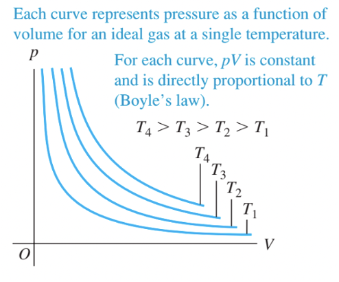
Fig. 3 Isotherms, or fixed-temperature curves, for a constant amount of an ideal gas. Source: Fig 18.6 from University Physics with Modern Physics (Pearson)

Example 3.2

Question

Find the variation in atmospheric pressure with elevation in the Earth’s atmosphere. You may assume that T = 0\(^{\circ}\) C and \(g\) = 9.8 m/s\(^2\) at all elevations.

Solution

For a fluid in equilibrium \(\frac{dP}{dy} = - \rho g\) where \(y\) is the elevation. Using \(m_{\rm total} = n M\) the ideal gas law can be expressed as \( PV = \frac{m_{total}}{M} RT \) so \(\rho = \frac{m_{total}}{V} = \frac{PM}{RT}.\) We can substitute for density and integrate \(\int \frac{1}{P} dP = -\frac{Mg}{RT} \int dy\) from sea level \((P_{0}, y_{0}\)) to elevation (\(P_{1}, y_{1}\)) \(\ln \frac{P_1}{P_0} = - \frac{Mg}{RT} (y_1 - y_0)\) so \(P_1 = P_0 \exp \left( - \frac{Mg}{RT} (y_1 - y_0) \right)\).

Pressure decreases exponentially with elevation. Setting \(P_0\) = 101 kPa and \(y_0\) = 0, we can evaluate the pressure at the summit of Everest (\(y_1\) = 8.86 x 10\(^3\) m). The atmosphere is predominantly N\(_2\) (amu = 28) and O\(_2\) (amu = 32) the mass of a mole of atmosphere is 29 g, so \(M g y_1/(RT) = 1.10\) and \(P_1 = 1.10 \times 10^{5} \exp (-1.10) = 3.4 \times 10^{4}\) Pa = 0.33 atm. This explains why mountaineers require oxygen, and jet planes required pressurised cabins.

The kinetic theory of the ideal gas

Suppose we have a box of volume \(V\) containing \(N\) molecules of an ideal gas. A molecule hits a wall of the container and bounces off it perfectly elastically, as shown in Fig. 4. The result of this is that the \(x\) component of the velocity of the particle reverses direction, but the \(y\) and \(z\) components don’t change, so the change in the momentum of the particle is \(\Delta p_m = 2 m |v_x|\) where \(m\) is the mass of the molecule.

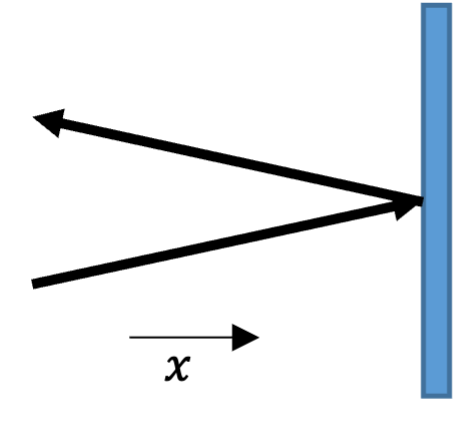
Fig. 4 A gas molecule bouncing off a wall

Kinetic theory deals in averages, so we need to work out the average number of molecules that hit the wall in some small time \(\Delta t\). Our molecule with \(x\)- velocity \(v_x\) will travel a distance \(v_x \Delta t\) in the \(x\) direction during this time, so it can hit the wall only if it is within this distance and is travelling in the right direction (a 50% chance, if its motion is random). Therefore the probability that it will hit the wall during the period in question is

\[ \frac{1}{2} A | v_{x} | \frac{\Delta t}{V} \]

where \(A\) is the area of the wall. Whenever it does hit the wall, its momentum changes by \(2 m|v_x|\), so by conservation of momentum it must impart an impulse \(2m|v_x|\) to the wall. Therefore the average force exerted by this molecule on the wall is

\[ \frac{\Delta p_{m}}{\Delta t} = \frac{m v_{x}^{2} A}{V}. \]

Summing over all the \(N\) molecules and dividing through by the area gives

(14)\[P = \frac{1}{A} \frac{dp}{dt} = \frac{N m <v_{x}^{2}>}{V}\]

where \(<v_x^2>\) is the mean square velocity in the \(x\) direction and the pressure \(P\) is the force per unit area. But if the molecules are moving in random directions we must have

\[ <v_x^{2}> = <v_y^{2}> = <v_z^{2}> = \frac{1}{3}<v^{2}> \]

because there is no preferred direction and \(v^2 = v_x^{2} + v_y^{2} = v_z^{3}\).

Therefore we obtain

(15)\[PV = \frac{1}{3} Nm<v^{2}> = \frac{2}{3} N <\frac{1}{2} m v^{2}>\]

where \(<1/2 m v^2>\) is the average kinetic energy of a gas molecule.

If we compare Equations (12) and (15) we see that

(16)\[<\frac{1}{2} m v^2 > = \frac{3}{2} k_{B} T.\]

This justifies the statement we made earlier, that temperature is a measure of the average kinetic energy of molecules. It should be noted that we are only considering translational kinetic energy here: molecules made of more than one atom may have internal kinetic energy relating to rotational or vibrational motion.

If we write the mean square velocity in terms of its components we have

(17)\[<\frac{1}{2} m v_{x}^{2}> = <\frac{1}{2} m v_{y}^{2}> = <\frac{1}{2} m v_{z}^{2}> = \frac{1}{2} k_{B} T.\]

Each individual component of the motion contributes \(1/2 k_B T\) to the total thermal energy. The principle of equipartition of energy states that every independent degree of freedom, i.e. quadratic term in the total energy, should have an equal share of the total - so, since each translational degree of freedom contributes \(1/2 k_B T\), any additional degrees of freedom, such as the rotational and vibrational motion we just mentioned, should do the same. This has interesting implications for the heat capacity, as we shall see below.

The thermal (kinetic) energy, \(K\), of the Sun is

\[ K = \frac{3}{2} k_{B} T N \]

where \(N = M_{\odot}/m_{p}\) is the number of particles (assuming purely hydrogen), \(M_{\odot}\) is the Solar mass, and \(m_{p} = 1.67 \times 10^{-27}\) kg is the proton mass.

The gravitational potential energy, \(U\), of the Sun, under the simplifying assumption of a uniform density sphere, is

\[ U = -\frac{3 G M_{\odot}^{2}}{5 R_{\odot}} \]

where \(R_{\odot}\) is the radius of the Sun.

From statistical physics, the Virial theorem states that

\[ 2K + U = 0 \]

for an body in equilibrium, i.e. the sum of twice the kinetic energy plus the potential energy is zero. From the Virial theorem we can evaluate the average temperature of the Sun

\[ T = \frac{G M_{\odot} m_{p}}{5 k_{B} R_{\odot}} = 4.6 \times 10^{6} {\rm K}. \]

The Maxwell-Boltzmann distribution

The temperature of an ideal gas defined the average kinetic energy of its molecules, according to Equation (16). However, the energies of the individual molecules actually span a wide range. This is described by the Maxwell-Boltzmann distribution of molecular speeds, which shown in Fig. 5 and mathematically is expressed as

(18)\[f(v) = \frac{4}{\sqrt\pi} \left( \frac{m}{2 k_{B} T} \right)^{3/2} v^2 \exp \left( -\frac{m v^{2}}{2 k_{B} T}\right).\]

Here \(f(v)\) is the probability that a molecule has a speed between \(v\) and \(v+dv\), \(m\) is the mass of the molecule, and \(T\) is the temperature. The factor \(\exp (-mv^{2}/2k_{B}T)\), which is the negative exponential of the relevant energy (in this case \(\frac{1}{2} m v^2\)) divided by \(k_B T\) is called a Boltzmann factor. Boltzmann factors occur frequently in thermodynamics and statistical mechanics, for example in the Saha equation in astrophysics. It can be derived using statistical mechanics.

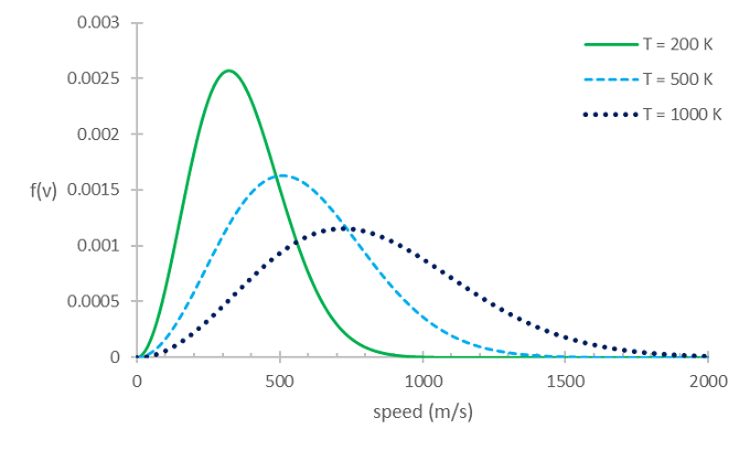
Fig. 5 Maxwell-Boltzmann distribution for O\(_2\) at three different temperatures

Properties of the Maxwell-Boltzmann distribution

The following derivation is not examinable (that would be mean)

We already know that \(<m v^2> = 3 k_B T\) from Equation (16) so it must be true that \(<v^2> = 3 k_B T/m\). The most probable value of \(v\) can be found by differentiating Equation (18) and setting the derivative to zero.

\[ \frac{df}{dv} = \frac{4}{\sqrt{\pi}} \left( \frac{m}{2 k_{B} T}\right)^{3/2} \left[ 2 v \exp \left( -\frac{mv^{2}}{2 k_{B} T}\right) - \frac{v^{3} m}{k_{B} T} \exp \left( - \frac{m v^2}{2 k_{B} T}\right) \right] \]

using the product role. This is zero for \(v = 0\), which is not useful, and for \(2 v = \frac{v^{3} m}{k_{B} T}\) which gives \(v_{\rm max} = \sqrt{2 k_{B}T/m}.\) Finally, since \(f(v)\) is a probability distribution, we can find the expectation value of \(v\) from

\[ <v> = \int_{0}^{\infty} v f(v)dv = \frac{4}{\sqrt{\pi}} \left( \frac{m}{2 k_{B}T}\right)^{3/2} \int_{0}^{\infty} v^{3} \exp \left( -\frac{m v^{2}}{2 k_{B} T} \right) dv. \]

This looks nasty but isn’t: if we write \(\alpha = m/(2 k_{B}T)\) for convenience and change variables to \(x = v^2\), we have

\[ \int_{0}^{\infty} v^{3} \exp \left( -\frac{m v^{2}}{2 k_{B} T}\right) dv = \frac{1}{2} \int_{0}^{\infty} x e^{-\alpha x} dx, \]

and this can be done by parts to get

\[ \frac{1}{2} \int_{0}^{\infty} x e^{-\alpha x} dx = \frac{1}{2} \left[ -\frac{1}{\alpha} x e^{-\alpha x}\right]_{0}^{\infty} + \frac{1}{2\alpha} \int_{0}^{\infty} e^{-\alpha x} dx = \frac{1}{2\alpha} \left[ -\frac{1}{\alpha} e^{-\alpha x}\right]_{0}^{\infty} = \frac{1}{2\alpha^2} = \frac{2 k_{B}^{2} T^{2}}{m^{2}}. \]

Therefore \(<v> = \sqrt{8 k_{B} T/\pi m}\). So in conclusion

(19)\[v_{\rm max} = \sqrt{ \frac{2 k_{B} T}{m}}; <v> = \sqrt{\frac{8 k_{B} T}{\pi m}}; v_{\rm rms} = \sqrt{<v^{2}>} = \sqrt{\frac{3 k_{B} T}{m}}.\]

Since \(2 < 8/\pi < 3,\) these are in increasing order: the root-mean-square speed is greater than the mean speed, which in turn is greater than the most probable speed. This is because the distribution has a long tail out to high speeds. From kinetic theory (Eqn (16)) we obtained \(<\frac{1}{2} m v^{2}> = \frac{3}{2} k_{B} T\) so \(<v^{2}> = v_{\rm rms}\) and is more commonly used than the most probable or mean - greater weight is given to higher speeds.

Example 3.3

Question

What is the most probable, mean and rms speed of oxygen molecules at room temperature (20\(^{\circ}\) C)?

Solution

The mass of a hydrogen atom (1 proton) is \(1.67 \times 10^{-27}\) kg, so oxygen (8 protons and neutrons) has a mass of \(2.67 \times 10^{-26}\) kg and diatomic oxygen has \(m = 5.34 \times 10^{-26}\) kg. Inserting \(T\) = 293 K and \(k_B = 1.38 \times 10^{-23}\) J/K into Eqn (19) yields \(v_{\rm max} = 390 {\rm m/s}; <v> = 440 {\rm m/s}; v_{\rm rms} = 480 {\rm m/s}.\) Light elements (H, He) have much higher speeds, so have largely escaped from low surface gravity environments such as the Earth (unlike gas giants Jupiter and Saturn).

Mean free path

In reality, gas molecules have finite sizes, so may collide with one another. We can estimate the frequency of collisions and distance travelled between collisions, by considering \(N\) spherical, identical molecules of radius \(r\) in a volume \(V\). Considering the motion of a single molecule, with speed \(v\), it will collide with another molecule as it sweeps out a cylinder of radius \(2r\), with it axis parallel to its motion - see Fig. 6. In time \(dt\) it will travel a distance \(v dt\) so collisions will occur within the volume \(4 \pi r^{2} v dt.\) There are \(N/V\) molecules per unit volume so the number \(dN\) with centres in the cylinder are \(dN = 4 \pi r^{2} v dt \frac{N}{V}\), So the number of collisions per unit time is \(\frac{dN}{dt} = 4 \pi r^{2} v \frac{N}{V}\). Considering the motion of all molecules is rather more involved, and results in a factor of \(\sqrt{2}\) more collisions \(\frac{dN}{dt} = 4\sqrt{2} \pi r^{2} v \frac{N}{V}\).

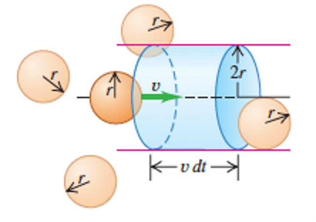
Fig. 6 In a time \(dt\) a molecule with radius \(r\) will collide with any other molecules within a cylindrical volume of radius \(2r\) and length \(v dt\). Source: Fig 18.15 from University Physics with Modern Physics (Pearson)

The average time \(t_{\rm mean}\) between collisions, the mean free time, is the recipricol of this expression \(t_{\rm mean} = \frac{V}{4 \sqrt{2} \pi r^{2} v N}\). The average distance travelled between collisions, the mean free path, denoted \(\lambda\), is the molecule’s speed multipled by \(t_{\rm mean}\)

(20)\[\lambda = v t_{\rm mean} = \frac{V}{4 \sqrt{2} \pi r^{2} N}.\]

The more molecules there are and the larger the molecule, the shorter the distance between collisions. Note that the mean free path does not depend on the speed of the molecule. We can also express the mean free path in terms of macroscopic properties of the gas using the ideal gas equation \(PV = N k_B T\).

\[ \lambda = \frac{k_{B} T}{4 \sqrt{2} \pi r^{2} P}. \]

If the temperature is increased at constant pressure, the gas expands, so the average distance between molecules increases, so \(\lambda\) increases. If the pressure is increase at fixed temperature, the gas compresses and \(\lambda\) decreases.

We can estimate these quantities for an oxygen molecule (\(r = 2.0 \times 10^{-10}\) m) at a pressure of 1 atm and temperature of 20\(^{\circ}\) C using \(v = v_{\rm rms}\) from Example 3.3. We obtain \(\lambda= 5.6 \times 10^{-8}\) m and \(t_{\rm mean} = 1.2 \times 10^{-10}\) s. A typical molecule undergoes nearly 10 billion collisions per second.

Heat capacity of ideal gases and equipartition of energy

If we supply heat to a gas at constant volume and raise its temperature by an amount \(\Delta T\), by definition we have supplied heat \(Q = nc\Delta T\), where \(n\) is the number of moles and \(c\) is the molar heat capacity. Equation (16) says that if we raise the temperature of n moles of an ideal gas by an amount \(\Delta T\), we increase the kinetic energy of its molecules by an amount

\[ \frac{3}{2} N k_{B} \Delta T = \frac{3}{2} nR\Delta T. \]

Equating these two, we conclude that

(21)\[c_{V} = \frac{3}{2} R. \]

However, there are some subtleties that we have to consider here.

1. In Equation (21) we have specified the molar heat capacity at constant volume. This is because if we heat the gas at constant volume, the heat energy supplied cannot do anything except increase the internal energy of the gas. This would not be true if we did not keep the volume constant: for example, if we heat the gas at constant pressure, it will expand, and this means that the gas pressure will do work on the surroundings of the gas.

2. We have assumed that the gas molecules have only translational kinetic energy, so if we add heat \(Q\) it is just divided equally among the three components of the particle velocity as in Equation (17). This will be true of monatomic gases like helium and neon. It is not true of more complicated molecules.

Heat capacity of a diatomic gas

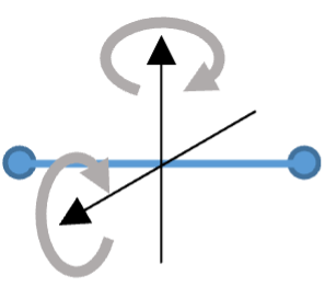
Fig. 7 Rotation of a diatomic molecule

Let’s consider a diatomic gas such as oxygen or nitrogen as two atoms joined by a bond, as illustrated in Fig. 7. Each molecule can move in three dimensions: it has three translational degrees of freedom. It can also rotate about either of two axes perpendicular to the line joining the atoms (rotation around the axis joining the two atoms doesn’t count, because in an ideal gas we assume the atoms have negligible size, so such a rotation is invisible): it has two rotational degrees of freedom. In addition the bond between the two atoms can behave like a spring: the atomis can vibrate to and fro along the line joining them. As the energy associated with this has two quadratic terms, \(1/2 k x^2\) (where k is the spring constant) for the potential energy and \(1/2 m v_{\rm vib}^2\) for the kinetic energy, it counts as two degrees of freedom, We therefore conclude that the total number of degrees of freedom is 3 + 2 + 2 = 7, and so raising the temperature of a mole of such a gas by an amount \(\Delta T\) should required

\[ Q = \frac{7}{2} N_{A} k_{B} \Delta T, \]

and therefore the molar heat capacity of a diatomic gas at constant volume should be \(c_{V} = 7/2 R\).

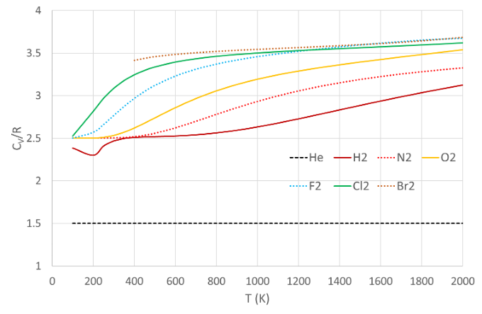
Fig. 8 Molar heat capacities of some diatomic gases, as a function of temperature. Data from NIST-JANAF thermochemical tables

However we see from Fig. 8 that this is not so. The molar heat capacity of helium (and other noble gases) behaves as we expect, but the diatomic gases approach \(7/2 R\) only at high temperatures. At room temperature common diatomic gases such as hydrogen, nitrogen and oxygen have \(c_{V} = \frac{5}{2} R\) - see Table 5.

Table entries from Table 18.1 of University Physics with Modern Physics (Pearson)

Table 5 Molar heat capacities of gases at room temperature

Gas	\(C_{V}\) J mol\(^{-1}\) K\(^{-1}\)	\(R\)
He	12.47	1.50
Ar	12.47	1.50
H\(_{2}\)	20.42	2.46
N\(_{2}\)	20.76	2.50
O\(_{2}\)	20.85	2.51
CO	20.85	2.51
CO\(_{2}\)	28.46	3.42
SO\(_{2}\)	31.39	3.78

The reason for this turns out to be quantum mechanical. Vibration and rotation are both quantized, and the first excited vibrational state is too high to reach at room temperature for most gases. Therefore the vibrational degrees of freedom are frozen out and the gas behaves as if it had 5 degrees of freedom (three translational and two rotational). The spacing of the vibrational energy levels is inversely proportional to the square root of the mass, which explains why heavy diatomic molecules like bromide do behave as if they have 7 degrees of freedom. Fig. 9 shows the experimental values of \(C_{V}\) for molecular hydrogen, which is representative of light diatomic molecules, requiring very high temperatures in order that \(C_{V} \sim 7/2 R\).

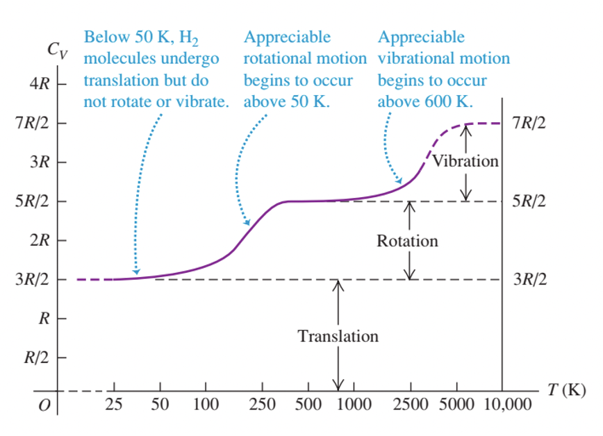
Fig. 9 Experimental values of \(C_{V}\) for \(H_{2}\) gas. Source: Fig 18.19 from University Physics with Modern Physics (Pearson)

Heat capacity of solids

We can extend the idea of equipartition of energy to solid materials. If we model a solid as a set of atoms in a crystal lattice joined by springs, each atomic can vibrate in three dimensions which means it has six degrees of freedom. We therefore predict that the molar heat capacity of a solid should be \(3 R\) (independent of temperature). This is the Dulong-Petit law, first found experimentally in 1819 by the French physicists Pierre Louis Dulong and Alexis Therese Petit. At room temperature, it is obeyed quite well for some solids (e.g. lead); however, as with diatomic gases, the heat capacities of solids show a temperature dependence that is not predicted by the model. Improved models can be constructed using the principles of statistical mechanics: you will look into this next year.

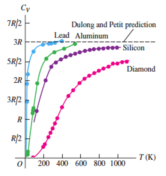
Fig. 10 Experimental values of \(C_{V}\) for lead, aluminium, silicon and diamond. Source: Fig 18.21 from University Physics with Modern Physics

Example 3.4

Question

The specific heat capacity of isobutane (C\(_4\) H\(_{10}\)) at constant volume is 1.477 kJ/kg/K at room temperature. How many rotational and vibrational degrees of freedom are active in this molecule?

Solution

The molar weight of isobutane is \(4 \times 12 + 10\) = 58 g. Its molar hear capacity is therefore 1477 x 0.058 = 85.66 J/mol/K. This is equal to \(\frac{f}{2} R\), where \(f\) is the total number of degrees of freedom. Dividing 85.66 by \(R/2\) gives \(f\) = 20.6. We subtract 3 for the translational kinetic energy degrees of freedom and get 17.6, which indicates that 17 degrees of freedom are completely active, and one is partially active (we can see from Fig. 8 that the transition from \(n\) to \(n+1\) degrees of freedom is not sharp - it is possible to be in between. This is because the molecules in a gas do not all have the same energy - recall Fig. 5.).